Main SPLAT module
The primary SPLAT module contains the definition of the core Spectrum object and associated function, standard classification and spectral analysis routines, and helper functions.
The SPLAT Spectrum object
Spectal data are manipulated as a Spectrum class object, which contains the relevant data (wavelength, flux, uncertainty) and additional information on the source and/or observation. A Spectrum object is the output of the various database access routines:
>>> import splat
>>> import splat.model as spmod
>>> sp = splat.getSpectrum(shortname='0415-0935')[0]    # note that getSpectrum returns a list
>>> sp = splat.getStandard('M0')[0]
>>> sp = spmod.getModel(teff = 700, logg=4.5)
>>> splist = splat.getSpectrum(spt=['M7','L5'],jmag=[14.,99.])
You can also read in your own spectrum by passing a filename
>>> sp = splat.Spectrum(filename='PATH_TO/myspectrum.fits')
Note that this file must conform to the standard of the SPL data: the first column is wavelength in microns, second column flux in F_lambda units, third column (optional) is flux uncertainty. The file can be a fits or ascii file.
You can also access a file based on its unique spectum key
>>> sp = splat.Spectrum(10002)
There are many aspects of the Spectrum class that can be referenced or set, all of which are described in the API entry. Some primary examples:
sp.wave,sp.flux,sp.noiseWavelengths, flux density (per wavelength) values, and flux uncertainty of the spectrum (uncertainty = NaN for models)
sp.wunit,sp.funitAstropy units for wavelength and flux, by default microns and erg/cm:sup: 2/s/micron
sp.nu,sp.fnu,sp.fnu_unitFrequencies, flux density (per frequency), and fnu units, by default Jy
sp.snrMedian estimate of spectrum signal-to-noise
sp.headerFits header (dictionary) from original file, if present
sp.teff,sp.logg,sp.z,sp.fsed,sp.cld,sp.kzzIf Spectrum is a model, these values give the effective temperature (in K), log surface gravity (cm/s2), log metallicity (relative to Sun), sedimentation efficient f:sub: sed(for Saumon & Marley 2012 models), cloud coverage fraction (for Morley models) and non-equilibrium chemistry diffusion constant
Built-in Commands
Information on the Spectrum object
The info() command produces a summary of the Spectrum object's primary information:
>>> sp.info()
The showHistory() command provides a summary of actions taken to maniupate a Spectrum object:
>>> sp.showHistory()
If you make changes to your Spectrum object, you can in many cases return it to its original state using the reset() function
>>> sp.reset()
To display the spectrum, use the Spectrum object's plot function, which makes use of the many options available in the plotSpectrum routine
>>> sp.plot()
>>> sp.plot(label='Awesome source', telluric=True)
>>> sp.plot(file='plot_output.eps')
You can save this display by adding a filename:
>>> sp.plot(sp,file='spectrum.png')
Saving a spectrum
A spectrum contained in a Spectrum object can be output to a file using the built-in export() or save() commands; both fits and tab-delimited ascii outputs are supported:
>>> sp.save('myspectrum.fits')
Spectral Analysis
SPLAT has several routines to do basic spectral analysis and combining of spectra.
Scaling a spectrum
Spectra can be scaled by an arbitrary factor:
>>> sp.scale(1.e9)
or simply normalized:
>>> sp.normalize()
Spectral math
Spectrum objects can be manipulated through normal arithmetic operations, which function on a wavelength-by-wavelength scale and properly propogate uncertainties
>>> sp3 = sp1+sp2
>>> sp3 = sp1-sp2
>>> sp3 = sp1*sp2
>>> sp3 = sp1/sp2
Comparing spectra
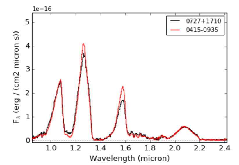
Spectra can be formally compared to each other using the compareSpectra() routine, which take two spectra and returns a comparison statistic and the optimal scale factor for the second spectrum:
>>> import splat
>>> sp7 = splat.getSpectrum(shortname='0727+1710')[0]
Retrieving 1 file
>>> sp8 = splat.getSpectrum(shortname='0415-0935')[0]
Retrieving 1 file
>>> chi,scale = splat.compareSpectra(sp7,sp8)
(20919.310008422835 0.766057330307)
>>> sp8.scale(scale)
>>> splat.plotSpectrum(sp7,sp8,colors=['k','r'],legend=['0727+1710','0415-0935'])
You can select different statistics usign the statistic keyword:
chisqr: chi squared value (requires spectra with noise values)
stddev: standard deviation
stddev_norm: normalized standard deviation
absdev: absolute deviation
- You can also tailor the wavelength ranges over which the spectra are compared by using one of the keywords:
fit_ranges= a nested set of 2-element arrays specifying which areas to fitmask_ranges= a nested set of 2-element arrays specifying which areas to avoidmask= an array of 0s (good) and 1s (bad) specifying the regions to fit; this can be generated using the generateMask() mask routinemask_telluricset to True masks the regions of strong telluric absorptionmask_standardset to True masks the telluric regions and wavelengths < 0.8 micron or > 2.35 micron
You can also weight the individual spectral pixels by passing an array to the weight keyword.
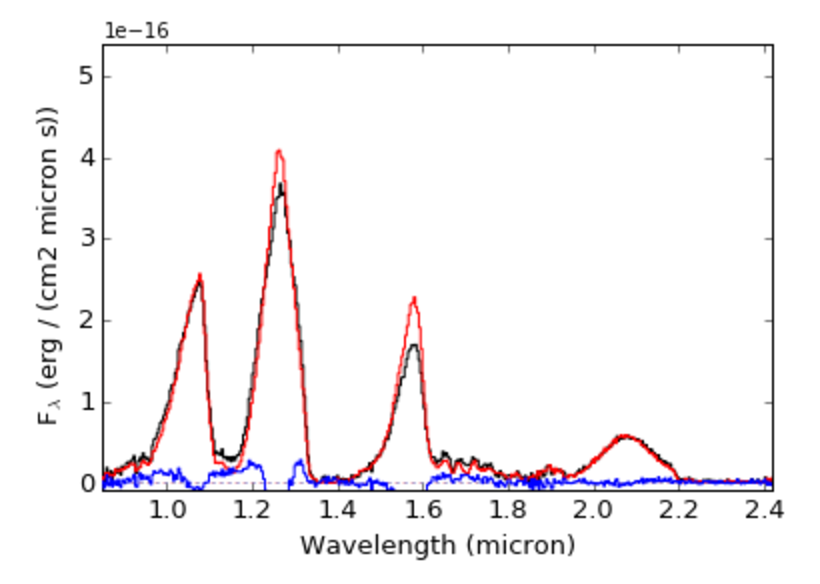
compareSpectra() has its own plotting output which can be triggered by setting plot to True. This will display the two spectra properly scaled and the difference spectra
>>> splat.compareSpectra(sp7,sp8,plot=True,mask_telluric=True)
(20670.083806484316 0.766085949716)
Reddening a spectrum
You can redden a spectrum following the Cardelli, Clayton, and Mathis (1989) reddening function using the redden() routine contained in the splat.empirical package:
>>> import splat
>>> sp = splat.Spectrum(10001)                   # read in a source
>>> sp.redden(sp,av=5.,rv=3.2)                          # redden to equivalent of AV=5
>>> splat.plotSpectrum(sp,spr,colors=['k','r'])
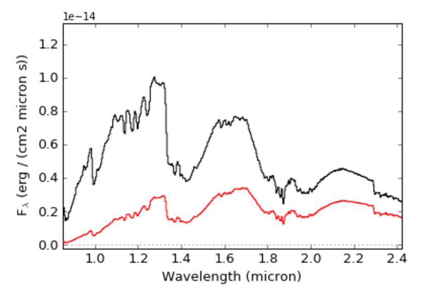
Here av is the visual reddening and rv the extinction coefficient (A_V = R_V * E(B-V) ), which is by default = 3.1, but can be modified (as in example above).
Spectrophotometry
SPLAT allows spectrophotometry of spectra using common filters in the red optical and near-infrared. The filter transmission files are stored in the SPLAT reference library, and are accessed by name. A list of current filters can be made by through the filterInfo() routine:
>>> import splat.photometry as sphot
>>> sphot.filterInfo()
  2MASS H: 2MASS H-band
  2MASS J: 2MASS J-band
  2MASS KS: 2MASS Ks-band
  BESSEL I: Bessel I-band
  FOURSTAR H: FOURSTAR H-band
  FOURSTAR H LONG: FOURSTAR H long
  ...
You can access specific information about a given filter profile with the filterProperties() routine
>>> result = sphot.filterProperties('2MASS J')
        Filter 2MASS J: 2MASS J-band
        Zeropoint = 1594.0 Jy
        Pivot point: = 1.252 micron
        FWHM = 0.280 micron
        Wavelength range = 1.075 to 1.416 micron
The filterMag() routine determines the photometric magnitude of a source based on its spectrum, by convolving fluxes with a defined filter profile:
>>> sp = splat.getSpectrum(shortname='1507-1627')[0]
>>> sp.fluxCalibrate('2MASS J',14.5)
>>> sphot.filterMag(sp,'MKO J')
    (14.346586427733005, 0.032091919093387822)
By default the filter is convolved with a model of Vega to extract Vega magnitudes, but the user can also set the ab parameter to get AB magnitudes, the photon parameter to get photon flux, or the energy parameter to get total energy flux:
>>> sphot.filterMag(sp,'MKO J',ab=True)
    (15.245064259793901, 0.031168695728282524)
>>> sphot.filterMag(sp,'MKO J',energy=True)
        (<Quantity 7.907663172914481e-13 erg / (cm2 s)>,
         <Quantity 2.090970538372485e-14 erg / (cm2 s)>)
>>> sphot.filterMag(sp,'MKO J',photon=True)
        (<Quantity 1.954421499626954e-24 1 / (cm2 s)>,
         <Quantity 5.53673880346918e-26 1 / (cm2 s)>)
One can measure photometry for custom filters using the custom parameter:
>>> import numpy
>>> fwave,ftrans = numpy.genfromtxt('my_custom_filter.txt',unpack=True)
>>> filt = numpy.vstack((fwave,ftans))
>>> sphot.filterMag(sp,'Custom',custom = filt)
        (13.097348489365396, 0.046530636178618558)
or define a simple notch filter with the two end wavelengthts:
>>> sphot.filterMag(sp,'Custom',notch=[1.2,1.3])
        (14.301864415761377, 0.031774478113182188)
Finally, to flux calibrate a spectrum to a given magnitude, use the Spectrum object's built in fluxCalibrate() method:
>>> sp.fluxCalibrate('2MASS J',14.0)
This routine can take absolute as a parameter flag to indicate that the spectra are absolutely flux calibrated:
>>> sp.fluxCalibrate('2MASS J',splat.typeToMag('L5','2MASS J')[0],absolute=True)
>>> sp.fscale
        'Absolute'
Classification
SPLAT contains several different methods for classifying a spectrum:
Classifying by Indices
SPLAT contains the spectral index/spectral type classification relations from the following studies:
These can be accessed through the classifyByIndices() routine, which returns the average subtype and uncertainty:
>>> sp = splat.getSpectrum(shortname='0559-1404')[0]
>>> splat.classifyByIndex(sp, string=True, set='burgasser', round=True)
        ('T4.5', 0.2562934083414341)
Using the allmeasures parameter provides the index values and individual index spectral types in a dictionary:
>>> sp = splat.getSpectrum(shortname='2320+4123')[0]
>>> splat.classifyByIndex(sp, set='reid', allmeasures=True)
        {'H2O-A': {'index': 0.76670417987511119,
          'index_e': 0.76670417987511119,
          'spt': 18.791162413674424,
          'spt_e': 1.1944901925036935},
         'H2O-B': {'index': 0.83184397268498511,
          'index_e': 0.83184397268498511,
          'spt': 19.956823648632948,
          'spt_e': 1.0460714823631427},
         'result': ('M9.5', 0.78695752933890462)}
Classifying by Standards
SPLAT contains spectral standards for dwarf classes M0 through T9, drawn from Burgasser et al. (2006), Kirkpatrick et al. (2010) and Cushing et al. (2011). There are also M and L subdwarf and M extreme subdwarf standards. These may be used to infer spectral classifications by "closest match", using all or part of the near-infrared spectrum.
The routine for this is classifyByStandard(), which by default simply matches to the best-fitting standard:
>>> sp = splat.getSpectrum(shortname='0805+4812')[0]
>>> splat.classifyByStandard(sp)
        ('T0.0', 0.5)
You can also return an uncertainty-weighted mean classifiction by setting average = True:
>>> splat.classifyByStandard(sp,average=True)
    ('L7.0::', 2.1064575737396338)
and fit to specific regions using either the fit_ranges parameter or setting method = 'kirkpatrick' to conform with the Kirkpatrick et al. (2010) method of near-infrared spectral classification:
>>> splat.classifyByStandard(sp,method='kirkpatrick')
    ('L7.0', 0.5)
Subdwarf and extreme subdwarf standards can be accessed by setting the sd, dsd or esd parameters to True.
Young spectral standards can be accessed by setting vlg, intg to True.
You can try all of these standards at once by setting all to True.
Finally, setting plot to True will bring up a comparison plot between the source and best fit standard.
>>> splat.classifyByStandard(sp,method='kirkpatrick',plot=True)
    ('L7.0', 0.5)

Note that the first time you run classifyByStandard(), the standards must be initially read in to the dictionaries splat.STDS_DWARF_SPEX, splat.STDS_SD_SPEX, splat.STDS_DSD_SPEX, splat.STDS_ESD_SPEX,
splat.STDS_VLG_SPEX and splat.STDS_INTG_SPEX. This can be prompted using the initiateStandards() routine:
>>> splat.initiateStandards()
One the standards are loaded, subsequent calls to classifyByStandard() are much faster.
Classifying by Templates
You can also classify sources by comparing to individual template spectra in the library. The classifyByTemplate() routine behaves similarly to `classifyByStandard`_, but has the option of returning a dictionary of the nbest best matches sorted by whatever statistic is desired (set with the statistic parameter; see compareSpectra()). Because each template must be read in, it is strongly recommended that users downselect the templates using keywords associated with searchLibrary():
>>> sp = splat.getSpectrum(shortname='1507-1627')[0]
>>> result = splat.classifyByTemplate(sp,spt=[24,26],nbest=5)
        Too many templates (1819) for classifyByTemplate; set force=True to override this
>>> result = splat.classifyByTemplate(sp,spt=[24,26],nbest=5)
    Too many templates (210) for classifyByTemplate; set force=True to override this
>>> result = splat.classifyByTemplate(sp,spt=[24,26],snr=80,nbest=5,verbose=True)
    Comparing to 58 templates
    LHS 102B L5.0 10488.1100432 11.0947838116
    SDSS J001608.44-004302.3 L5.5 15468.6209466 274.797693706
        2MASS J00250365+4759191AB L4.0 28458.3112163 4.19176819291
        2MASS J00332386-1521309 L4.0 29141.2681221 2.2567421444e-14
    ...
    Best match = DENIS-P J153941.96-052042.4 with spectral type L4:
    Mean spectral type = L4.5+/-0.724296125146
Note that the program doesn't proceed automatically if there are more than 100 templates; you can override this using the force parameter:
>>> result = splat.classifyByTemplate(sp,spt=[24,26],nbest=5,force=True,verbose=True)
        Comparing to 210 templates
        This may take some time!
        SDSS J000112.18+153535.5 L4.0 24551.836698 14.3533608111
        SDSS J000250.98+245413.8 L5.5 15517.679593 51.274551132
        ...
        Best match = 2MASS J17461199+5034036 with spectral type L5
        Mean spectral type = L5.0+/-0.42094300506
- You can also downselect templates using the
selectparameter for the following predefined template sets: select = m dwarf: fit to M dwarfs only
select = l dwarf: fit to M dwarfs only
select = t dwarf: fit to M dwarfs only
select = vlm: fit to M7-T9 dwarfs
select = optical: only optical classifications
select = high sn: median S/N greater than 100
select = young: only young/low surface gravity dwarfs
select = companion: only companion dwarfs
select = subdwarf: only subdwarfs
select = single: only dwarfs not indicated a binaries
select = spectral binaries: only dwarfs indicated to be spectral binaries
select = standard: only spectral standards (in this case it is better to use the ``classifyByStandard``_ routine instead)
These sets can be combined:
>>> result = splat.classifyByTemplate(sp,select='l dwarfs, young',nbest=5,verbose=True)
        Comparing to 79 templates
        SDSS J000112.18+153535.5 L4.0 24551.836698 14.3533608111
        2MASS J00193927-3724392 L3.0 10299.0508807 16.2807901643
        2MASS J0028208+224905 L5.0 19350.1803596 12.281257449
        ...
        Best match = 2MASS J10224821+5825453 with spectral type L1beta
        Mean spectral type = L0.5+/-0.86022832423
Gravity Classification
The classifyGravity() routine uses the index-based method of Allers & Liu (2013) to determine gravity scores from VO, FeH, K I and H-band continuum indices.
>>> sp = splat.getSpectrum(shortname='1507-1627')[0]
>>> splat.classifyGravity(sp)
    FLD-G
In its default mode it also determines the classification of the source using the
Allers et al. (2007) index-based scheme, but you can also force an spectral type by setting the spt parameter:
>>> splat.classifyGravity(sp,spt='L5')
    FLD-G
Finally, the routine will return a dictionary of all index scores by setting the allscores parameter to True:
>>> result = splat.classifyGravity(sp, allscores = True, verbose=True)
    Gravity Classification:
        SpT = L4.0
        VO-z: 1.012+/-0.029 => 0.0
        FeH-z: 1.299+/-0.031 => 1.0
        H-cont: 0.859+/-0.032 => 0.0
        KI-J: 1.114+/-0.038 => 1.0
        Gravity Class = FLD-G
>>> print(result)
    {'FeH-z': 1.0,
     'H-cont': 0.0,
     'KI-J': 1.0,
     'VO-z': 0.0,
     'gravity_class': 'FLD-G',
     'score': 0.5,
     'spt': 'L4.0'}
Useful Program Constants
splat.DB_SOURCESA pandas table containing the Source Database
splat.DB_SPECTRAA pandas table containing the Spectrum Database
splat.STDS_DWARF_SPEX, splat.STDS_SD_SPEX, splat.STDS_DSD_SPEX, splat.STDS_ESD_SPEX,
splat.STDS_VLG_SPEX and splat.STDS_INTG_SPEX
Dictionaries containing Spectrum objects of the SpeX classification standard templates; this dictionary is populated through calls to `splat.getStandard()`_ . A standard Spectrum object can be accessed by using the spectral type as the referring key:
>>> sp = splat.getStandard('M0')[0]                 # both are Spectrum objects of Gliese 270
>>> sp = splat.STDS_DWARF_SPEX['M0.0']          # note the mandatory decimal
splat.FILTERSA dictionary containing information on all of the filters used in SPLAT photometry.
splat.INSTRUMENTSA dictionary containing information on the instruments currently read in as native to the SPLAT code.
splat.SPECTRAL_MODELSA dictionary containing information on the spectral models currently contained in the SPLAT code
splat.EVOLUTIONARY_MODELSA dictionary containing information on the evolutionary models currently contained in the SPLAT code
Search