SPLAT Plotting Routines
The SPLAT plotting routines are designed to visualize spectral data and comparisons to other templates and models. These are all contained in the splat.plot module, which should be imported separately:
>>> import splat.plot as splot
Basic spectral plots
The core plotting function is plotSpectrum(), which allows flexible methods for displaying single or groups of spectra, and comparing spectra to each other. Nearly all of the functions described below are wrappers for plotSpectrum() with various options, described in more detail in the API. Plots are made using the pyplot package in matplotlib.
The simplest way to visualize a spectrum is to simply call plotSpectrum() with the Spectrum class object:
>>> import splat
>>> import splat.plot as splot
>>> spc = splat.getSpectrum(spt = 'T5', lucky=True)[0]
>>> splot.plotspectrum(spc)
You can also use the Spectrum class's built in plot() function:
>>> spc.plot()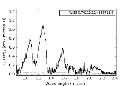
Note that this adds a legend with the name of the source, the uncertainty spectrum (if present) and the zeropoint. These can be called explicitly within plotSpectrum() as well:
>>> splot.plotspectrum(spc,legend=spc.name,showNoise=True,showZero=True)
There are many options for adding details to your spectrum plot, listed below. In addition, the output of a call to plotSpectrum() is a matplotlib.figure.Figure class
>>> plt = splat.plotspectrum(spc)
>>> plt
  [<matplotlib.figure.Figure at 0x119e4f710>]
so you can use other options from this class to further augment your plot.
Feature labels and legends
Specific absorption features can be labeled on the plot by setting the features to a list of atoms and molecules.
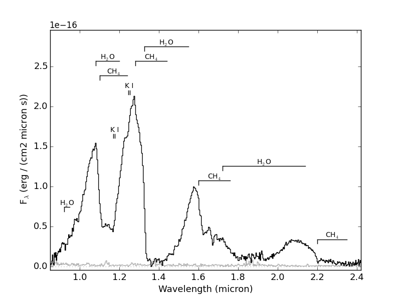
>>> spc = splat.getSpectrum(spt = 'T5', lucky=True)[0]
>>> splot.plotSpectrum(spc,features=['h2o','ch4','h2'])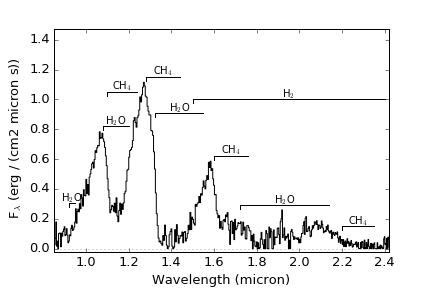
The features currently contained in the code include:
- Lines:
H I lines at 1.004, 1.093, 1.281, 1.944, and 2.166 micron
Na I: lines at 0.819, 1.136, and 2.21 micron
K I: lines at 0.767, 0.770, 1.169, 1.177, 1.244 and 1.252 micron
Ca I: lines at 1.931, 1.946, 1.951, 1.978, 1.986, 1.987, 2.263, and 2.265 micron
Ca II: lines at 0.986, 0.993, 1.184, and 1.195 micron
Mg I: lines at 1.183, 1.209, 1.488, 1.503, 1.504, 1.575, 1.576, and 1.711 micron
Al I: lines at 1.313, 1.315, 1.672 and 1.676 micron
Fe I: lines at 1.143, 1.160, 1.161, 1.164, 1.169, 1.189, 1.198, 1.256, 1.288 and 1.501 micron
- Molecules:
H2O: bands at 0.92-0.95, 1.08-1.20, 1.33-1.55, and 1.72-2.14 micron
CO: band at 2.29-2.39
TiO: bands at 0.76-0.80 and 0.825-0.831 micron
VO: band at 1.04-1.08 micron
FeH: bands at 0.98-1.03, 1.19-1.25, and 1.57-1.64 micron
CH4: bands at 1.10-1.24, 1.28-1.44, 1.60-1.76, and 2.20-2.35 micron
H2: broad absorption over 1.5-2.4 micron
SB: the spectral binary feature between 1.60-1.64 micron
You can also set groups of features based on the type of object; options include mdwarf, ldwarf and tdwarf
>>> spc = splat.getSpectrum(spt = 'L5', lucky=True)[0]
>>> splot.plotSpectrum(spc,ldwarf=True)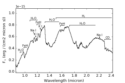
To label and shade regions of telluric absorption, set telluric = True
>>> splot.plotSpectrum(spc,telluric=True)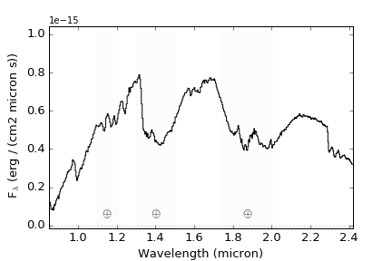
To add a legend, use the legend or label keyword:
>>> spc = splat.getSpectrum(lucky=True)[0]
>>> spt,spt_e = splat.classifyByStandard(spc)
>>> splot.plotSpectrum(spc,legend=['{} SpT = {}'.format(spc.shortname,spt)])
You can vary the size and location of the legend using the legendfontscale and legendlocation keywords.
Insets
You can place an inset in your plot to zoom in on a particular feature using the inset keyword:
>>> spc = splat.getSpectrum(sbinary=True, lucky=True)[0]
>>> spc.normalize()
>>> splot.plotSpectrum(spc,inset=True)
You can get some control over the positioning and sampled range using inset_position (left edge, bottom edge, width, height) and inset_xrange:
>>> splot.plotSpectrum(spc,inset=True,inset_xrange=[1.52,1.72],inset_position=[0.6,0.55,0.28,0.32])
Colors and line styles
plotSpectrum() uses the same commands as pyplot for setting colors (default black) and linestyles (default solid):
>>> spc = splat.getSpectrum(spt = 'M9', lucky=True)[0]
>>> splot.plotSpectrum(spc,color='red',linestyle=':')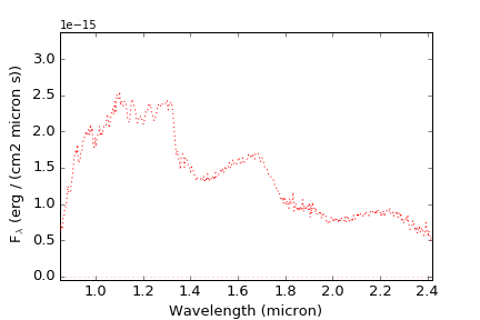
Manipulating the plot format
You can adjust the plot ranges using the xrange and yrange keywords
>>> spc = splat.getSpectrum(spt = 'T5', lucky=True)[0]
>>> spc.normalize()
>>> splot.plotSpectrum(spc,xrange=[1.0,1.6],yrange=[0,2])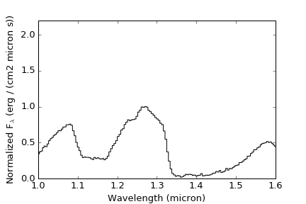
Or change the labels of these axes using the xlabel and ylabel keywords
>>> splot.plotSpectrum(spc,xrange=[1.0,1.6],yrange=[0,2],xlabel='A Length Quantity',ylabel='A Flux Density Quantity')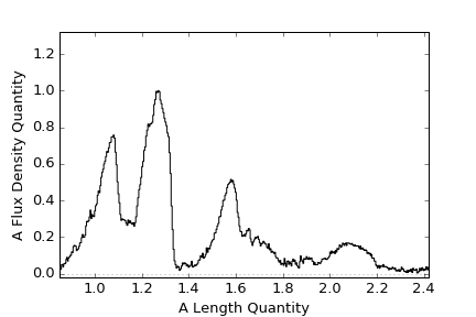
You can also adjust the plot size using the figsize keyword
>>> splot.plotSpectrum(spc,figsize=(12,4))
Exporting the plot
To export the plot to a file, simply set the file keyword:
>>> splot.plotSpectrum(spc,file='myplot.pdf')
Note that matplotlib automatically figures out the file format based on the filename suffix.
Plotting multiple spectra
plotSpectrum() can also manage plotting multiple spectra, either on top of each other or stacked in the plot, or across multiple. There are also separate routines to handle common cases.
Comparison plots
Spectra can be stacked on top of each other using the stack parameter, which is a numerical value that indicates the offset between sequential spectra. For example, the plot the sequence of NIR L dwarf standards:
>>> splat.initiateStandards()
>>> stdspt = [splat.typeToNum(i) for i in range(20,30)]
>>> sps = [splat.STDS_DWARF_SPEX[s] for s in stdspt]
>>>
[EXAMPLE NEEDED MULTIPLE SPECTRA]
[PLOTBATCH]
[PLOTSEQUENCE]
Multi-page plots
Other Plotting Tools
plotMap()
plotMap() plots coordinates onto a sky map, with options to plot groups of coordinates with different colors, symbols, and symbol sizes. plotMap() takes as its primary input an array of astropy Skycoord objects, but will do conversions as necesssary with properCoordinates(). Map projections are those defined in the matplotlib Basemap documentation.
For example, to plot all of the sources labeled "young" in the SPLAT library:
>>> s = splat.searchLibrary(young=True)
>>> c = [splat.properCoordinates(x) for x in s['DESIGNATION']]
>>> splot.plotMap(c)
Or to plot bright M dwarfs and L dwarfs separately, and save to a file:
>>> sm = splat.searchLibrary(spt=['M0','M9.5'],jmag=13)
>>> sl = splat.searchLibrary(spt=['L0','L9.5'],jmag=13)
>>> cm = [splat.properCoordinates(x) for x in sm['DESIGNATION']]
>>> cl = [splat.properCoordinates(x) for x in sm['DESIGNATION']]
>>> splot.plotMap(cm,cl,colors=['k','r'],markers=['o','o'],alpha=[0.3,0.9],output='bright_ml_map.pdf')
Examples
- Example 1: A simple view of a random spectrum
This example shows various ways of displaying a random spectrum in the library
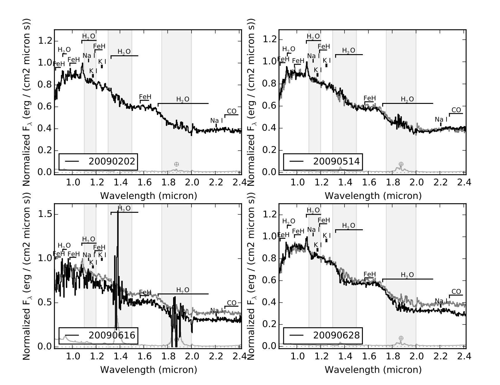
>>> import splat
>>> spc = splat.getSpectrum(spt = 'T5', lucky=True)[0]   # select random spectrum
>>> spc.`plot()`                                                 # this automatically generates a "quicklook" plot
>>> splat.plotSpectrum(spc)                                      # does the same thing
>>> splat.plotSpectrum(spc,uncertainty=True,tdwarf=True)     # show the spectrum uncertainty and T dwarf absorption features
The last plot should look like the following:
- Example 2: Compare two spectra
Optimally scale and compare two spectra.
>>> import splat
>>> spc = splat.getSpectrum(spt = 'T5', lucky=True)[0]   # select random spectrum
>>> spc2 = splat.getSpectrum(spt = 'T4', lucky=True)[0]  # read in another random spectrum
>>> comp = splat.compareSpectra(spc,spc2)        # compare spectra to get optimal scaling
>>> spc2.scale(comp[1])                  # apply optimal scaling
>>> splat.plotSpectrum(spc,spc2,colors=['black','red'],labels=[spc.name,spc2.name])     # show the spectrum uncertainty and T dwarf absorption features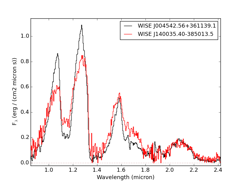
- Example 3: Compare several spectra for a given object
In this case we'll look at all of the spectra of TWA 30B in the library, sorted by year and compare each to the first epoch data. This is an example of using both multiplot and multipage.
>>> splist = splat.getSpectrum(name = 'TWA 30B')         # get all spectra of TWA 30B
>>> junk = [sp.normalize() for sp in splist]             # normalize the spectra
>>> dates = [sp.date for sp in splist]                   # observation dates
>>> spsort = [s for (d,s) in sorted(zip(dates,splist))]   # sort spectra by dates
>>> dates.sort()                                         # don't forget to sort dates!
>>> splat.plotSpectrum(spsort,multiplot=True,layout=[2,2],multipage=True,\   # here's our plot statement
    comparison=spsort[0],uncertainty=True,mdwarf=True,telluric=True,legends=dates,\
    legendLocation='lower left',output='TWA30B.pdf')
Here is the first page of the resulting 5 page pdf file
- Example 4: Display the spectra sequence of L dwarfs
This example uses the list of standard files contained in SPLAT, and illustrates the stack feature
>>> spt = [splat.typeToNum(i+20) for i in range(10)] # generate list of L spectral types
>>> splat.initiateStandards()                        # initiate standards
>>> splist = [splat.SPEX_STDS[s] for s in spt]       # extact just L dwarfs
>>> junk = [sp.normalize() for sp in splist]         # normalize the spectra
>>> labels = [sp.shortname for sp in splist]         # set labels to be names
>>> splat.plotSpectrum(splist,figsize=[10,20],labels=labels,stack=0.5,\  # here's our plot statement
    colorScheme='copper',legendLocation='outside',telluric=True,output='lstandards.pdf')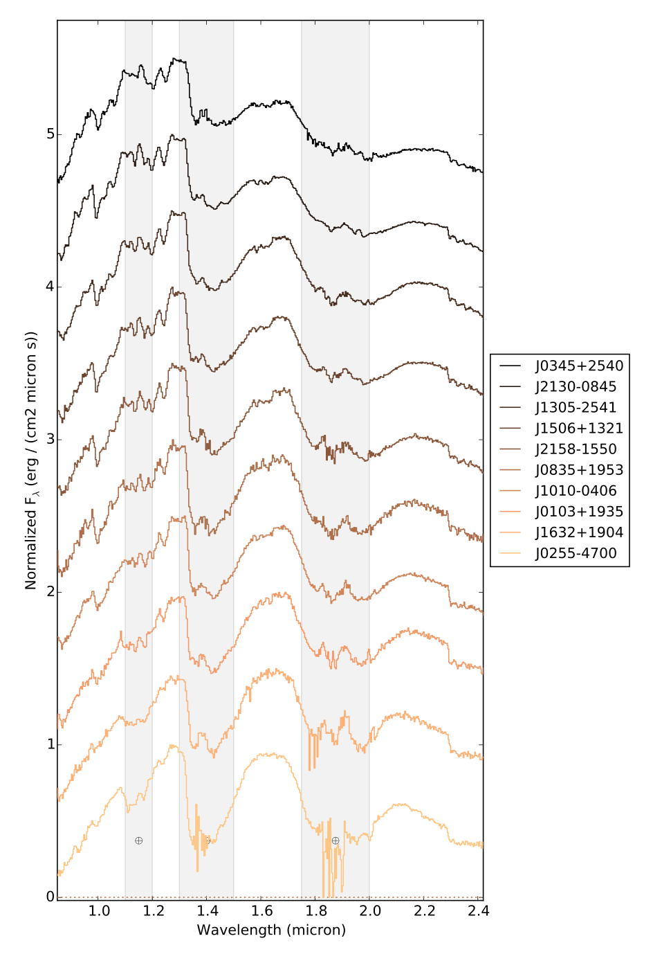
Search